A linear combination is a sum of scaled vectors

vmls-note-5.md still pointed at the opening definition on printed page 15, and 05-scalar.md still had the properties I had checked entry by entry. I stayed in the same Desktop folder in BaseHalf 0.7.0 and kept reading, now from printed page 17.

This is part 6 of the close reading of Boyd and Vandenberghe's Introduction to Applied Linear Algebra. I did not start a new canvas. A linear combination is a name for a sum I could already form, once I had addition and scalar multiplication.

A note grown from the definition of a linear combination

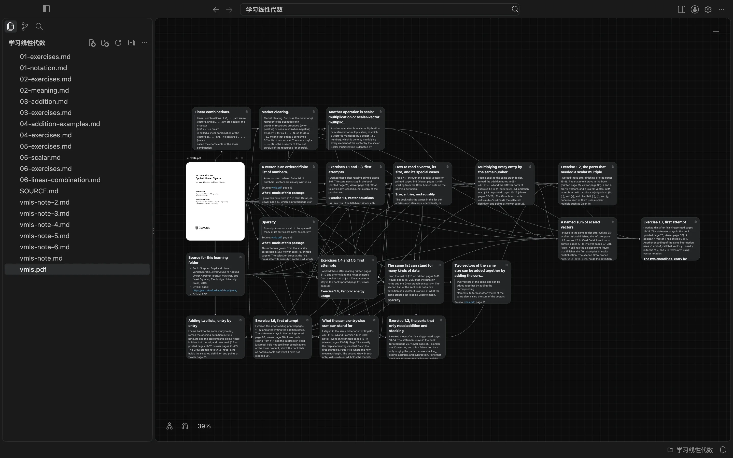
In Card Detail I went to viewer page 27, printed page 17, selected the definition of a linear combination, and chose Grow branch, again from the reader, not from the cover. The new file was vmls-note-6.md. It already listed vmls.pdf as upstream and pointed at page 27.

The first block of the selection is complete: if a_1, …, a_m are n-vectors and β_1, …, β_m are scalars, the vector β_1 a_1 + ··· + β_m a_m is a linear combination of those vectors, and the scalars are its coefficients. The selection then runs on into the next heading, "Linear combination of unit vectors," and stops at a line break, so the note ends at "as a linea." I am not treating the cut line as the whole sentence.

I checked the definition on two 2-vectors of my own. If a_1 = (1, 0) and a_2 = (0, 2), then 0.5 a_1 + 3 a_2 = (0.5, 0) + (0, 6) = (0.5, 6).

The book then writes any n-vector as a linear combination of the standard unit vectors: b = b_1 e_1 + ··· + b_n e_n. The coefficients are the entries of b, and e_i is the ith unit vector I already had in 01-notation.md. I checked this on b = (2, −1, 0): 2 e_1 + (−1) e_2 + 0 e_3 is (2, 0, 0) + (0, −1, 0) + (0, 0, 0) = (2, −1, 0). I also followed the book's own 3-vector example on that page, and it matched the same pattern.

Special names, and what the same sum can stand for

I wrote the rest into 06-linear-combination.md, with the book, the new Grow branch note, and the scalar-multiplication notes as upstream.

Some choices of coefficients have names. If every coefficient is 1, the linear combination is the sum. If every coefficient is 1/m, it is the average, which I can also write as (1/m)(a_1 + ··· + a_m). If the coefficients themselves add up to 1, it is an affine combination. If those coefficients are also nonnegative, it is a convex combination, a mixture, or a weighted average. The book notes that those coefficients are sometimes written as percentages that add up to 100%.

I checked the average on the same pair: (1/2)(a_1 + a_2) = (1/2)(1, 2) = (0.5, 1). For an affine combination that is not an average, (1 − 0.25) a_1 + 0.25 a_2 = 0.75(1, 0) + 0.25(0, 2) = (0.75, 0.5), and 0.75 + 0.25 = 1.

On printed page 18 the meanings begin. If the vectors are displacements, a linear combination is the sum of the scaled displacements. If they are audio tracks recorded over the same period, the linear combination is a mix, and the loudness of each track follows |β_i|.

Cash flow replication uses the same arithmetic. The book gives two one-period loans of $1 with 10% interest, c_1 = (1, −1.1, 0) and c_2 = (0, 1, −1.1). I computed d = c_1 + 1.1 c_2 myself: 1.1 c_2 = (0, 1.1, −1.21), and c_1 + 1.1 c_2 = (1, 0, −1.21). That is a two-period loan of $1 in period 1, with the interest compounded. The 0 in the middle is the point: the repayment of the first loan is exactly the start of the second.

The last example is a line and a segment. For two different n-vectors a and b, the affine combination c = (1 − θ)a + θb lies on the line through a and b. When 0 ≤ θ ≤ 1, c is a convex combination and lies on the segment between them. The book says this still makes sense when the vectors are 100-dimensional, not only when they are coordinates in the plane. I checked it on a pair of my own, a = (0, 0) and b = (4, 2): θ = 0 gives a, θ = 1 gives b, θ = 1/2 gives (2, 1), and θ = 1.2 gives (4.8, 2.4), which is past b on the same line. Figure 1.12, which illustrates those values of θ, sits at the top of the next printed page, where §1.4 begins. I looked at the figure and did not start the inner product.

Exercise 1.7

The attempt is in 06-exercises.md. The statement stays in the book, on printed page 26. A Boolean n-vector x has entries 0 or 1. Another encoding of the same information uses −1 and +1; call that vector y. I needed y in terms of x, and x in terms of y.

If x_i = 0, then y_i should be −1. If x_i = 1, then y_i should be +1. The arithmetic that does that to a single number is y_i = 2x_i − 1. The same rule on every entry is

y = 2x − 1

where 1 is the ones vector of the same size as x. That is also a linear combination of x and 1, with coefficients 2 and −1. Going back, x = (1/2)(y + 1).

I first used a short list of my own, x = (1, 0, 1). Then 2x − 1 = (1, −1, 1), and (1/2)((1, −1, 1) + (1, 1, 1)) = (1, 0, 1), which is x again. I also applied the same formulas to the 4-vector given in the exercise, and the result matched the alternative encoding written there.

I checked this against the definition of scalar-vector multiplication in vmls-note-5.md, the ones vector in 01-notation.md, and the linear combination in vmls-note-6.md, not against a solution key. I did not ask an agent to grade it in this session.

What stays for the next section

vmls-note-6.md, 06-linear-combination.md, and 06-exercises.md now sit in the same folder as the definition of scalar multiplication and the leftover parts of Exercise 1.2. §1.3 is finished only in the sense that I have read the section and tried a representative exercise that needs it. The inner product is still next.

This is part 6 of Learning applied linear algebra with BaseHalf, a close reading of Introduction to Applied Linear Algebra. Previous: Multiplying a vector by a number scales every entry.